Using Bio-Formats in MATLAB
This section assumes that you have installed the MATLAB toolbox as instructed in the MATLAB user information page. Note the minimum recommended MATLAB version is R2017b.
As described in Using Java Libraries, every installation of MATLAB includes a JVM allowing use of the Java API and third-party Java libraries. All the helper functions included in the MATLAB toolbox make use of the Bio-Formats Java API. Please refer to the Javadocs for more information.
Increasing JVM memory settings
The default JVM settings in MATLAB can result in
java.lang.OutOfMemoryError: Java heap space exceptions when opening large
image files using Bio-Formats. Information about the Java heap space usage in
MATLAB can be retrieved using:
java.lang.Runtime.getRuntime.maxMemory
MATLAB Preferences (R2010a+)
Default JVM settings can be increased by Java Heap Memory Preferences of MATLAB (R2010a onwards) using . We recommend to use 512 MB in general, but you don’t need to decrease the value if the default value is bigger than 512 MB.
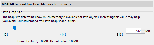
However, the maximum value allowed in the Preferences GUI (typically set to 25% of Physical Memory, whihc you can ask by the memory MATLAB command) can still be too small
for your purpose. In that case, you can directly edit matlab.prf file in the
folder specified by the prefdir MATLAB function
(eg. 'C:\Users\xxxxxxx\AppData\Roaming\MathWorks\MATLAB\R2018b'). Find the
parameter JavaMemHeapMax in the file and increase the number that follows
the capital I (in MB) to increase the maximum Java heap memory size. The
change will be reflected by the Preferences as above.
JavaMemHeapMax=I25000
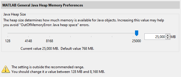
You will see a warning message as above.
java.opts
Alternatively, this can also be done by creating a java.opts file in
the startup directory
and overriding the default memory settings (see this page
for more information). We recommend using -Xmx512m (meaning 512 MB) in your java.opts
file.
Calling:
bfCheckJavaMemory()
will also throw a warning if the runtime memory is lower than the recommended value.
If errors of type java.lang.OutOfMemoryError: PermGen space are thrown
while using Bio-Formats with the Java bundled with MATLAB, you
may try to increase the default values of -XX:MaxPermSize and
-XX:PermSize via the java.opts file.
Opening an image file
The first thing to do is initialize a file with the bfopen function:
data = bfopen('/path/to/data/file');
This function returns an n-by-4 cell array, where n is the number of
series in the dataset. If s is the series index between 1 and n:
The
data{s, 1}element is anm-by-2 cell array, wheremis the number of planes in thes-th series. Iftis the plane index between 1 andm:The
data{s, 1}{t, 1}element contains the pixel data for thet-th plane in thes-th series.The
data{s, 1}{t, 2}element contains the label for thet-th plane in thes-th series.
The
data{s, 2}element contains original metadata key/value pairs that apply to thes-th series.The
data{s, 3}element contains color lookup tables for each plane in thes-th series.The
data{s, 4}element contains a standardized OME metadata structure, which is the same regardless of the input file format, and contains common metadata values such as physical pixel sizes - see OME metadata below for examples.
Accessing planes
Here is an example of how to unwrap specific image planes for easy access:
seriesCount = size(data, 1);
series1 = data{1, 1};
series2 = data{2, 1};
series3 = data{3, 1};
metadataList = data{1, 2};
% etc
series1_planeCount = size(series1, 1);
series1_plane1 = series1{1, 1};
series1_label1 = series1{1, 2};
series1_plane2 = series1{2, 1};
series1_label2 = series1{2, 2};
series1_plane3 = series1{3, 1};
series1_label3 = series1{3, 2};
Displaying images
If you want to display one of the images, you can do so as follows:
series1_colorMap1 = data{1, 3}{1, 1};
figure('Name', series1_label1);
if isempty(series1_colorMap1)
  colormap(gray);
else
  colormap(series1_colorMap1);
end
imagesc(series1_plane1);
This will display the first image of the first series with its associated
color map (if present). If you would prefer not to apply the color maps
associated with each image, simply comment out the calls to colormap.
If you have the image processing toolbox, you could instead use:
imshow(series1_plane1, []);
You can also create an animated movie (assumes 8-bit unsigned data):
cmap = gray(256);
for p = 1 : size(series1, 1)
  M(p) = im2frame(uint8(series1{p, 1}), cmap);
end
if feature('ShowFigureWindows')
  movie(M);
end
Retrieving metadata
There are two kinds of metadata:
Original metadata is a set of key/value pairs specific to the input format of the data. It is stored in the
data{s, 2}element of the data structure returned bybfopen.OME metadata is a standardized metadata structure, which is the same regardless of input file format. It is stored in the
data{s, 4}element of the data structure returned bybfopen, and contains common metadata values such as physical pixel sizes, instrument settings, and much more. See the OME Model and Formats documentation for full details.
Original metadata
To retrieve the metadata value for specific keys:
% Query some metadata fields (keys are format-dependent)
metadata = data{1, 2};
subject = metadata.get('Subject');
title = metadata.get('Title');
To print out all of the metadata key/value pairs for the first series:
metadataKeys = metadata.keySet().iterator();
for i=1:metadata.size()
  key = metadataKeys.nextElement();
  value = metadata.get(key);
  fprintf('%s = %s\n', key, value)
end
OME metadata
Conversion of metadata to the OME standard is one of Bio-Formats’ primary features. The OME metadata is always stored the same way, regardless of input file format.
To access physical voxel and stack sizes of the data:
omeMeta = data{1, 4};
stackSizeX = omeMeta.getPixelsSizeX(0).getValue(); % image width, pixels
stackSizeY = omeMeta.getPixelsSizeY(0).getValue(); % image height, pixels
stackSizeZ = omeMeta.getPixelsSizeZ(0).getValue(); % number of Z slices

voxelSizeXdefaultValue = omeMeta.getPixelsPhysicalSizeX(0).value();           % returns value in default unit
voxelSizeXdefaultUnit = omeMeta.getPixelsPhysicalSizeX(0).unit().getSymbol(); % returns the default unit type
voxelSizeX = omeMeta.getPixelsPhysicalSizeX(0).value(ome.units.UNITS.MICROMETER); % in µm
voxelSizeXdouble = voxelSizeX.doubleValue();                                  % The numeric value represented by this object after conversion to type double
voxelSizeY = omeMeta.getPixelsPhysicalSizeY(0).value(ome.units.UNITS.MICROMETER); % in µm
voxelSizeYdouble = voxelSizeY.doubleValue();                                  % The numeric value represented by this object after conversion to type double
voxelSizeZ = omeMeta.getPixelsPhysicalSizeZ(0).value(ome.units.UNITS.MICROMETER); % in µm
voxelSizeZdouble = voxelSizeZ.doubleValue();                                  % The numeric value represented by this object after conversion to type double
For more information about the methods to retrieve the metadata, see the MetadataRetrieve Javadoc page.
To convert the OME metadata into a string, use the dumpXML() method:
omeXML = char(omeMeta.dumpXML());
Changing the logging level
By default, bfopen uses bfInitLogging to initialize the logging system
at the WARN level. To change the root logging level, use the
DebugTools methods as
described in the Logging section.
% Set the logging level to DEBUG
loci.common.DebugTools.setRootLevel('DEBUG');
Reading from an image file
The main inconvenience of the bfopen.m function is that it loads all the content of an image regardless of its size.
To access the file reader without loading all the data, use the low-level bfGetReader.m function:
reader = bfGetReader('path/to/data/file');
You can then access the OME metadata using the getMetadataStore()
method:
omeMeta = reader.getMetadataStore();
Individual planes can be queried using the bfGetPlane.m function:
series1_plane1 = bfGetPlane(reader, 1);
To switch between series in a multi-image file, use the setSeries(int) method. To retrieve a plane given a set of (z, c, t) coordinates, these coordinates must be linearized first using getIndex(int, int, int)
% Read plane from series iSeries at Z, C, T coordinates (iZ, iC, iT)
% All indices are expected to be 1-based
reader.setSeries(iSeries - 1);
iPlane = reader.getIndex(iZ - 1, iC -1, iT - 1) + 1;
I = bfGetPlane(reader, iPlane);
Saving files
The basic code for saving a 5D array into an OME-TIFF file is located in the bfsave.m function.
For instance, the following code will save a single image of 64 pixels by 64 pixels with 8 unsigned bits per pixels:
plane = zeros(64, 64, 'uint8');
bfsave(plane, 'single-plane.ome.tiff');
And the following code snippet will produce an image of 64 pixels by 64 pixels with 2 channels and 2 timepoints:
plane = zeros(64, 64, 1, 2, 2, 'uint8');
bfsave(plane, 'multiple-planes.ome.tiff');
By default, bfsave will create a minimal OME-XML metadata object
containing basic information such as the pixel dimensions, the dimension order
and the pixel type.
To customize the OME metadata, it is possible to create a metadata object
from the input array using createMinimalOMEXMLMetadata.m, add custom
metadata and pass this object directly to bfsave:
plane = zeros(64, 64, 1, 2, 2, 'uint8');
metadata = createMinimalOMEXMLMetadata(plane);
pixelSize = ome.units.quantity.Length(java.lang.Double(.05), ome.units.UNITS.MICROMETER);
metadata.setPixelsPhysicalSizeX(pixelSize, 0);
metadata.setPixelsPhysicalSizeY(pixelSize, 0);
pixelSizeZ = ome.units.quantity.Length(java.lang.Double(.2), ome.units.UNITS.MICROMETER);
metadata.setPixelsPhysicalSizeZ(pixelSizeZ, 0);
bfsave(plane, 'metadata.ome.tiff', 'metadata', metadata);
The dimension order of the file on disk can be specified in two ways:
either by passing an OME-XML metadata option as a key/value pair as shown above
or as an optional positional argument of
bfsave
If a metadata object is passed to bfsave, its dimension order stored
internally will take precedence.
For more information about the methods to store the metadata, see the MetadataStore Javadoc page.
Improving reading performance
Initializing a Bio-Formats reader can consume substantial time and memory. Most of the initialization time is spend in the setId(java.lang.String) call. Various factors can impact the performance of this step including the file size, the amount of metadata in the image and also the file format itself.
One solution to improve reading performance is to use Bio-Formats memoization functionalities with the loci.formats.Memoizer reader wrapper. By essence, the speedup gained from memoization will only happen after the first initialization of the reader for a particular file.
The simplest way to make use the Memoizer functionalities in MATLAB is
illustrated by the following example:
% Construct an empty Bio-Formats reader
r = bfGetReader();
% Decorate the reader with the Memoizer wrapper
r = loci.formats.Memoizer(r);
% Initialize the reader with an input file
% If the call is longer than a minimal time, the initialized reader will
% be cached in a file under the same directory as the initial file
% name .large_file.bfmemo
r.setId(pathToFile);

% Perform work using the reader

% Close the reader
r.close()

% If the reader has been cached in the call above, re-initializing the
% reader will use the memo file and complete much faster especially for
% large data
r.setId(pathToFile);

% Perform additional work

% Close the reader
r.close()
If the time required to call setId(java.lang.String) method is larger
than DEFAULT_MINIMUM_ELAPSED or the minimum value
passed in the constructor, the initialized reader will be cached in a memo
file under the same folder as the input file. Any subsequent call to
setId() with a reader decorated by the Memoizer on the same input file
will load the reader from the memo file instead of performing a full reader
initialization.
More constructors are described in the Memoizer javadocs allowing to control the minimal initialization time required before caching the reader and/or to define a root directory under which the reader should be cached.
As Bio-Formats is not thread-safe, reader memoization offers a new solution to increase reading performance when doing parallel work. For instance, the following example shows how to combine memoization and MATLAB parfor to do work on a single file in a parallel loop:
% Construct a Bio-Formats reader decorated with the Memoizer wrapper
r = loci.formats.Memoizer(bfGetReader(), 0);
% Initialize the reader with an input file to cache the reader
r.setId(pathToFile);
% Close reader
r.close()

nWorkers = 4;

% Enter parallel loop
parfor i = 1 : nWorkers
    % Initialize logging at INFO level
    bfInitLogging('INFO');
    % Initialize a new reader per worker as Bio-Formats is not thread safe
    r2 = javaObject('loci.formats.Memoizer', bfGetReader(), 0);
    % Initialization should use the memo file cached before entering the
    % parallel loop
    r2.setId(pathToFile);

    % Perform work

    % Close the reader
    r2.close()
end
